Introduction

Why akid

Why another package on neural network?

Neural network, which is broadly named as Deep Learning nowadays, seems to have the potential to lead another technology revolution. It has incurred wide enthusiasm in industry, and serious consideration in public sector and impact evaluation in government. However, though being a remarkable breakthrough in high dimensional perception problems academically and intellectually stimulating and promising, it is still rather an immature technique that is fast moving and in shortage of understanding. Temporarily its true value lies in the capability to solve data analytic problems in industry, e.g. self-driving cars, detection of lung cancer etc. On the other hand, Neural Network is a technique that heavily relies on a large volume of data. It is critical for businesses that use such a technique to leverage on newly available data as soon as possible, which helps form a positive feedback loop that improves the quality of service.

Accordingly, to benefits from the newest development and newly available data, we want the gap between research and production as small as possible. In this package, we explore technology stacks abstraction that enable fast research prototyping and are production ready.

akid tries to provide a full stack of softwares that provides abstraction to let researchers focus on research instead of implementation, while at the same time the developed program can also be put into production seamlessly in a distributed environment, and be production ready when orchestrating with containers, a cluster manager, and a distributed network file system.

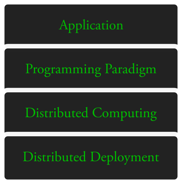
At the top application stack, it provides out-of-box tools for neural network applications. Lower down, akid provides programming paradigm that lets user easily build customized model. The distributed computing stack handles the concurrency and communication, thus letting models be trained or deployed to a single GPU, multiple GPUs, or a distributed environment without affecting how a model is specified in the programming paradigm stack. Lastly, the distributed deployment stack handles how the distributed computing is deployed, thus decoupling the research prototype environment with the actual production environment, and is able to dynamically allocate computing resources, so developments (Devs) and operations (Ops) could be separated.

akid stack

Now we discuss each stack provided by akid.

Application stack

At the top of the stack, akid could be used as a part of application without knowing the underlying mechanism of neural networks.

akid provides full machinery from preparing data, augmenting data, specifying computation graph (neural network architecture), choosing optimization algorithms, specifying parallel training scheme (data parallelism etc), logging and visualization.

Neural network training — A holistic example

To create better tools to train neural network has been at the core of the original motivation of akid. Consequently, in this section, we describe how akid can be used to train neural networks. Currently, all the other feature resolves around this.

The snippet below builds a simple neural network, and trains it using MNIST, the digit recognition dataset.

from akid import AKID_DATA_PATH
from akid import FeedSensor
from akid import Kid
from akid import MomentumKongFu
from akid import MNISTFeedSource

from akid.models.brains import LeNet

brain = LeNet(name="Brain")
source = MNISTFeedSource(name="Source",
                         url='http://yann.lecun.com/exdb/mnist/',
                         work_dir=AKID_DATA_PATH + '/mnist',
                         center=True,
                         scale=True,
                         num_train=50000,
                         num_val=10000)

sensor = FeedSensor(name='Sensor', source_in=source)
s = Kid(sensor,
        brain,
        MomentumKongFu(name="Kongfu"),
        max_steps=100)
kid.setup()
kid.practice()

It builds a computation graph as the following

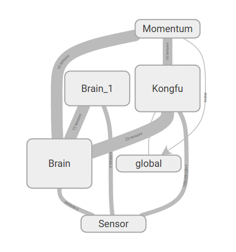
The story happens underlying are described in the following, which also debriefs the design motivation and vision behind.

akid is a kid who has the ability to keep practicing to improve itself. The kid perceives a data Source with its Sensor and certain learning methods (nicknamed KongFu) to improve itself (its Brain), to fulfill a certain purpose. The world is timed by a clock. It represents how long the kid has been practicing. Technically, the clock is the conventional training step.

To break things done, Sensor takes a Source which either provides data in form of tensors from Tensorflow or numpy arrays. Optionally, it can make jokers on the data using Joker, meaning doing data augmentation. The data processing engine, which is a deep neural network, is abstracted as a Brain. Brain is the name we give to the data processing system in living beings. A Brain incarnates one of data processing system topology, or in the terminology of neural network, network structure topology, such as a sequentially linked together layers, to process data. Available topology is defined in module systems. The network training methods, which are first order iterative optimization methods, is abstracted as a class KongFu. A living being needs to keep practicing Kong Fu to get better at tasks needed to survive.

A living being is abstracted as a Kid class, which assemblies all above classes together to play the game. The metaphor means by sensing more examples, with certain genre of Kong Fu(different training algorithms and policies), the data processing engine of the Kid, the brain, should get better at doing whatever task it is doing, letting it be image classification or something else.

Visualization

As a library gearing upon research, it also has rich features to visualize various components of a neural network. It has built-in training dynamics visualization, more specifically, distribution visualization on multi-dimensional tensors, e.g., weights, activation, biases, gradients, etc, and line graph visualization on on scalars, e.g., training loss, validation loss, learning rate decay, regularzation loss in each layer, sparsity of neuron activation etc, and filter and feature map visualization for neural networks.

Distribution and scalar visualization are built in for typical parameters and measures, and can be easily extended, and distributedly gathered. Typical visualization are shown below.

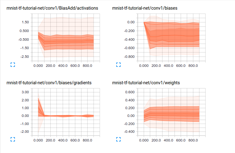
Visualization of how distribution of multi-dimensional tensors change over time. Each line on the chart represents a percentile in the distribution over the data: for example, the bottom line shows how the minimum value has changed over time, and the line in the middle shows how the median has changed. Reading from top to bottom, the lines have the following meaning: [maximum, 93%, 84%, 69%, 50%, 31%, 16%, 7%, minimum] These percentiles can also be viewed as standard deviation boundaries on a normal distribution: [maximum, μ+1.5σ, μ+σ, μ+0.5σ, μ, μ-0.5σ, μ-σ, μ-1.5σ, minimum] so that the colored regions, read from inside to outside, have widths [σ, 2σ, 3σ] respectively.

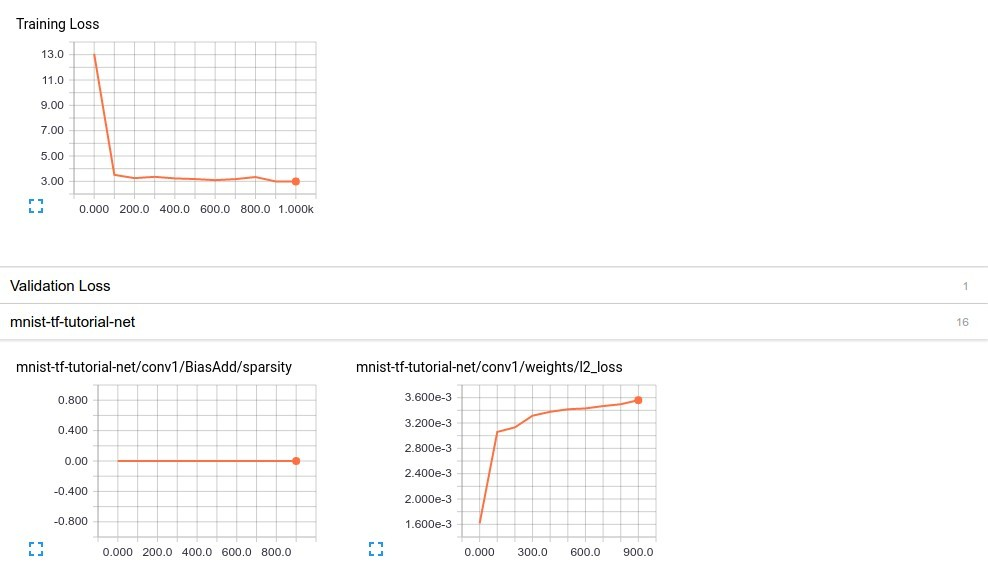
Visualization of how important scalar measures change over time.

akid supports visualization of all feature maps and filters with control on the layout through Observer class. When having finished creating a Kid, pass it to Observer, and call visualization as the following.

from akid import Observer

o = Observer(kid)
# Visualize filters as the following
o.visualize_filters()
# Or visualize feature maps as the following
o.visualize_activation()

Various layouts are provided when drawing the filters. Additional features are also available. The post-preprocessed results are shown below.

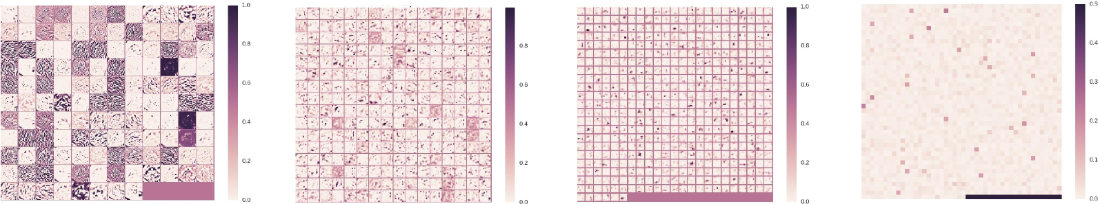
Visualization of feature maps learned.

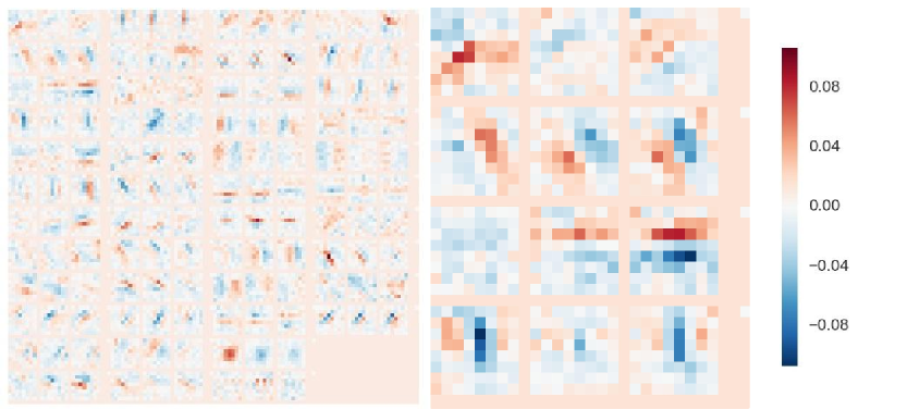
Visualization of filters learned.

Programming Paradigm

We have seen how to use functionality of akid without much programming in the previous section. In this section, we would like to introduce the programming paradigm underlying the previous example, and how to use akid as a research library with such paradigm.

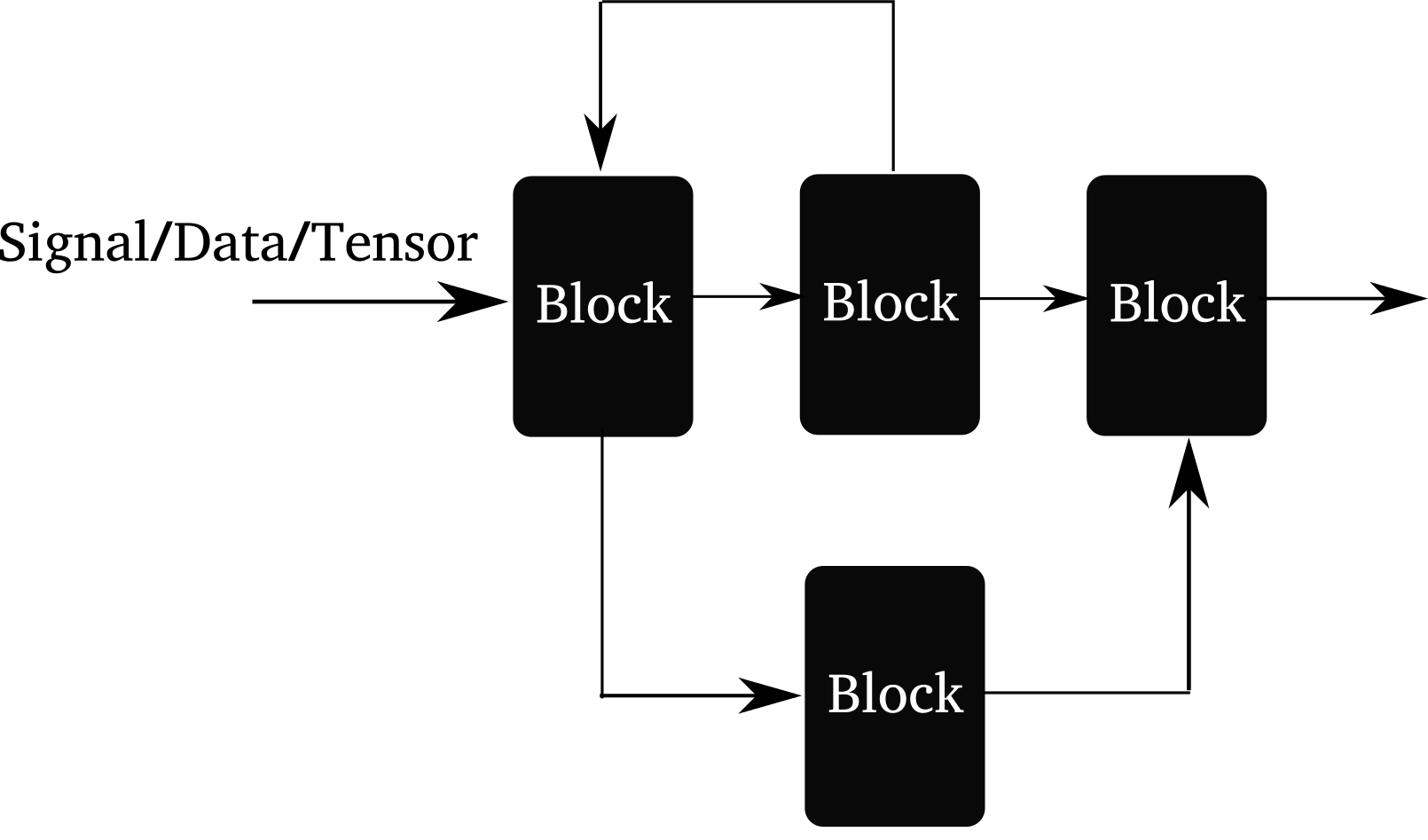
Illustration of the arbitrary connectivity supported by akid. Forward connection, branching and mergine, and feedback connection are supported.

akid builds another layer of abstraction on top of Tensor: Block. Tensor can be taken as the media/formalism signal propagates in digital world, while Block is the data processing entity that processes inputs and emits outputs.

It coincides with a branch of “ideology” called dataism that takes everything in this world is a data processing entity. An interesting one that may come from A Brief History of Tomorrow by Yuval Noah Harari.

Best designs mimic nature. akid tries to reproduce how signals in nature propagates. Information flow can be abstracted as data propagating through inter-connected blocks, each of which processes inputs and emits outputs. For example, a vision classification system is a block that takes image inputs and gives classification results. Everything is a Block in akid.

A block could be as simple as a convonlutional neural network layer that merely does convolution on the input data and outputs the results; it also be as complex as an acyclic graph that inter-connects blocks to build a neural network, or sequentially linked block system that does data augmentation.

Compared with pure symbol computation approach, like the one in tensorflow, a block is able to contain states associated with this processing unit. Signals are passed between blocks in form of tensors or list of tensors. Many heavy lifting has been done in the block (Block and its sub-classes), e.g. pre-condition setup, name scope maintenance, copy functionality for validation and copy functionality for distributed replicas, setting up and gathering visualization summaries, centralization of variable allocation, attaching debugging ops now and then etc.

akid offers various kinds of blocks that are able to connect to other blocks in an arbitrary way, as illustrated above. It is also easy to build one’s own blocks. The Kid class is essentially an assembler that assemblies blocks provided by akid to mainly fulfill the task to train neural networks. Here we show how to build an arbitrary acyclic graph of blocks, to illustrate how to use blocks in akid.

A brain is the data processing engine to process data supplied by Sensor to fulfill certain tasks. More specifically,

• it builds up blocks to form an arbitrary network
• offers sub-graphs for inference, loss, evaluation, summaries
• provides access to all data and parameters within

To use a brain, feed in data as a list, as how it is done in any other blocks. Some pre-specified brains are available under akid.models.brains. An example that sets up a brain using existing brains is:

# ... first get a feed sensor
sensor.setup()
brain = OneLayerBrain(name="brain")
input = [sensor.data(), sensor.labels()]
brain.setup(input)

Note in this case, data() and labels() of sensor returns tensors. It is not always the case. If it does not, saying return a list of tensors, you need do things like:

input = [sensor.data()]
input.extend(sensor.labels())

Act accordingly.

Similarly, all blocks work this way.

A brain provides easy ways to connect blocks. For example, a one layer brain can be built through the following:

class OneLayerBrain(Brain):
    def __init__(self, **kwargs):
        super(OneLayerBrain, self).__init__(**kwargs)
        self.attach(
            ConvolutionLayer(ksize=[5, 5],
                            strides=[1, 1, 1, 1],
                            padding="SAME",
                            out_channel_num=32,
                            name="conv1")
        )
        self.attach(ReLULayer(name="relu1"))
        self.attach(
            PoolingLayer(ksize=[1, 5, 5, 1],
                        strides=[1, 5, 5, 1],
                        padding="SAME",
                        name="pool1")
        )

        self.attach(InnerProductLayer(out_channel_num=10, name="ip1"))
        self.attach(SoftmaxWithLossLayer(
            class_num=10,
            inputs=[
                {"name": "ip1", "idxs": [0]},
                {"name": "system_in", "idxs": [1]}],
            name="loss"))

It assembles a convolution layer, a ReLU Layer, a pooling layer, an inner product layer and a loss layer. To attach a block (layer) that directly takes the outputs of the previous attached layer as inputs, just directly attach the block. If inputs exists, the brain will fetch corresponding tensors by name of the block attached and indices of the outputs of that layer. See the loss layer above for an example. Note that even though there are multiple inputs for the brain, the first attached layer of the brain will take the first of these input by default, given the convention that the first tensor is the data, and the remaining tensors are normally labels, which is not used till very late.

As an example to build more complex connectivity scheme, residual units can be built using Brain as shown below.

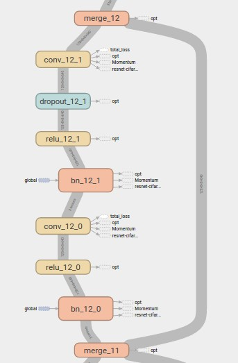
One residual units. On the left is the branch that builds up patterns complexity, and on the right is the stem branch that shorts any layers to any layer. They merge at the at the start and at the end of the branching points.

Parameter tuning

akid offers automatic parameter tuning through defining template using tune function.

akid.train.tuner.tune(template, opt_paras_list=[{}], net_paras_list=[{}], repeat_times=1, gpu_num_per_instance=1, debug=False)

A function tune that takes a Brain jinja2 template class and a parameters to fill the template in runtime. Parameters provided should complete the remaining network parameters in the template. The tuner is not aware of the content of the list items. It is up to the user to define template right, so parameters will be filled in the right place.

The jinja2 template must be a function named setup, and return a set up Kid. All necessary module imports should be put in the function instead of module level import usually.

The tune function would use all available GPUs to train networks with all given different set of parameters. If available GPUs are not enough, the ones that cannot be trained will wait till some others finish, and get its turn.

## Parameter Tuning Usage

Tunable parameters are divided into two set, network hyper parameters, net_paras_list, and optimization hyper parameters, opt_paras_list. Each set is specified by a list whose item is a dictionary that holds the actual value of whatever hyper parameters defined as jinja2 templates. Each item in the list corresponds to a tentative training instance. network paras and optimization paras combine with each other exponentially(or in Cartesian Product way if we could use Math terminology), which is to say if you have two items in network parameter list, and two in optimization parameters, the total number of training instances will be four.

Final training precisions will be returned as a list. Since the final precision normally will not be the optimal one, which normally occurs during training, the returned values are used for testing purpose only now

## Run repeated experiment

To run repeated experiment, just leave opt_paras_list and net_paras_list to their default value.

## GPU Resources Allocation

If the gpu_num_per_instance is None, a gpu would be allocated to each thread, otherwise, the length of the list should be the same with that of the training instance (aka the #opt_paras_list * #net_paras_list * repeat_times), or an int.

Given the available GPU numbers, a semaphore is created to control access to GPUs. A lock is created to control access to the mask to indicator which GPU is available. After a process has modified the gpu mask, it releases the lock immediately, so other process could access it. But the semaphore is still not release, since it is used to control access to the actual GPU. A training instance will be launched in a subshell using the GPU acquired. The semaphore is only released after the training has finished.

## Example

For example, to tune the activation function and learning rates of a network, first we set up network parameters in net_paras_list, optimization parameters in opt_paras_list, build a network in the setup function, then pass all of it to tune:

net_paras_list = []
net_paras_list.append({
    "activation": [
        {"type": "relu"},
        {"type": "relu"},
        {"type": "relu"},
        {"type": "relu"}],
    "bn": True})
net_paras_list.append({
    "activation": [
        {"type": "maxout", "group_size": 2},
        {"type": "maxout", "group_size": 2},
        {"type": "maxout", "group_size": 2},
        {"type": "maxout", "group_size": 5}],
    "bn": True})

opt_paras_list = []
opt_paras_list.append({"lr": 0.025})
opt_paras_list.append({"lr": 0.05})

def setup(graph):

    brain.attach(cnn_block(
        ksize=[8, 8],
        init_para={
            "name": "uniform",
            "range": 0.005},
        wd={"type": "l2", "scale": 0.0005},
        out_channel_num=384,
        pool_size=[4, 4],
        pool_stride=[2, 2],
        activation={{ net_paras["activation"][1] }},
        keep_prob=0.5,
        bn={{ net_paras["bn"] }}))

tune(setup, opt_paras_list, net_paras_list)

Distributed Computation

The distributed computing stack is responsible to handle concurrency and communication between different computing nodes, so the end user only needs to deal with how to build a power network. All complexity has been hidden in the class Engine. The usage of Engine is just to pick and use.

More specifically, akid offers built-in data parallel scheme in form of class Engine. Currently, the engine mainly works with neural network training, which is be used with Kid by specifying the engine at the construction of the kid.

As an example, we could do data parallelism on multiple computing towers using:

kid = kids.Kid(
    sensor,
    brain,
    MomentumKongFu(lr_scheme={"name": LearningRateScheme.placeholder}),
    engine={"name": "data_parallel", "num_gpu": 2},
    log_dir="log",
    max_epoch=200)

The end computational graph constructed is illustrated below

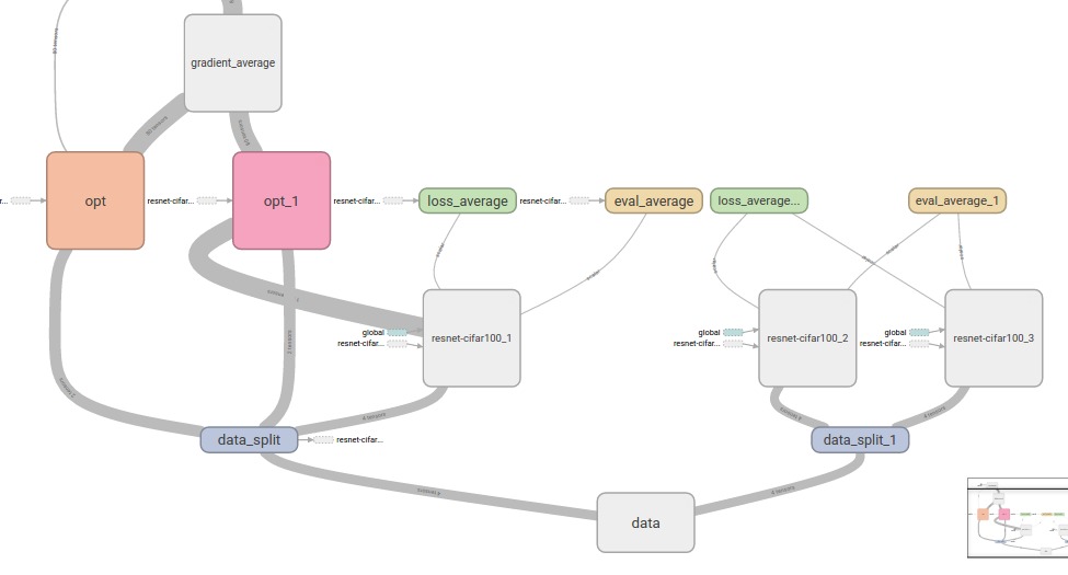
Illustration of computational graph constructed by a data parallel engine. It partitions a mini-batch of data into subsets, as indicated by the data_split blue blocks, and passes the subsets to replicates of neural network models at different coputing tower, as indicated by the gray blocks one level above blue blocks, then after the inference results have been computed, the results and the labels (from the splitted data block) will be passed to the optimizers in the same tower, as indicated by red and orange blocks named opt, to compute the gradients. Lastly, the gradients will be passed to an tower that computes the average of the gradients, and pass them back to neural networks of each computing towers to update their parameters.

Distributed Deployment

The distributed deployment stack handles the actual production environment, thus decouples the development/prototyping environment and production environment. Mostly, this stack is about how to orchestrate with existing distributed ecosystem. Tutorials will be provided when a production ready setup has been thoroughly investigated. Tentatively, glusterfs and Kubernetes are powerful candidates.

Comparison with existing packages

akid differs from existing packages from the perspective that it aims to integrate technology stacks to solve both research prototyping and industrial production. Existing packages mostly aim to solve problems in one of the stack. akid reduces the friction between different stacks with its unique features. We compare akid with existing packages in the following briefly.

Theano, Torch, Caffe, MXNet are packages that aim to provide a friendly front end to complex computation back-end that are written in C++. Theano is a python front end to a computational graph compiler, which has been largely superseded by Tensorflow in the compilation speed, flexibility, portability etc, while akid is built on of Tensorflow. MXNet is a competitive competitor to Tensorflow. Torch is similar with theano, but with the front-end language to be Lua, the choice of which is mostly motivated from the fact that it is much easier to interface with C using Lua than Python. It has been widely used before deep learning has reached wide popularity, but is mostly a quick solution to do research in neural networks when the integration with community and general purpose production programming are not pressing. Caffe is written in C++, whose friendly front-end, aka the text network configuration file, loses its affinity when the model goes more than dozens of layer.

DeepLearning4J is an industrial solution to neural networks written in Java and Scala, and is too heavy weight for research prototyping.

Perhaps the most similar package existing with akid is Keras, which both aim to provide a more intuitive interface to relatively low-level library, i.e. Tensorflow. akid is different from Keras at least two fundamental aspects. First, akid mimics how signals propagates in nature by abstracting everything as a semantic block, which holds many states, thus is able to provide a wide range of functionality in a easily customizable way, while Keras uses a functional API that directly manipulates tensors, which is a lower level of abstraction, e.g. it have to do class attributes traverse to retrieve layer weights with a fixed variable name while in akid variable are retrieved by names. Second, Keras mostly only provides an abstraction to build neural network topology, which is roughly the programming paradigm stack of akid, while akid provides unified abstraction that includes application stack, programming stack, and distributed computing stack. A noticeable improvement is Keras needs the user to handle communication and concurrency, while the distributed computing stack of akid hides them.